An EXAFS Scan
This is an example for an EXAFS scan.
Four counters are used.
It is demonstrated how
different steps widths are used in
different energy regions.
The scan is called by:
ONLINE scan/exafs
Table 15.13:
Example: EXAFS Scan Menu
                              --- EXAFS Scan ---
   SPECTRA>

   EXAFS:           8888.016      [eV]          A-Move:                    [eV]


-------------------------------------------------------------------------------
   Scan_Name:         ak_0016
   Generic Scan Name: ak
   Comment:
   Start:           8630          [eV]     Stop:         9900         [eV]
   Delta:           10            [eV]     Sample_time:  0.5          [Seconds]
   Range:                                  NP:
   Scan_par:        1                      Wait_time     0.
   Maximum x        0             [eV]     SSA:          No
   Auto-return:     (1) YES                Repeats:      1
-------------------------------------------------------------------------------
   Edit com-files
    <~.prog>before_fast_scan.gra                                      NO
    <~.prog>during_fast_scan.gra                                      NO
    <~.prog>after_fast_scan.gra                                       NO
-------------------------------------------------------------------------------
 PF1 - Start Scan, PF2 - Continue Scan, PF4 - Exit, <Space bar> - Stop Scan
 KP7 - Cursor scan_name, Z - Toggle Zoom, D - Display, ^W - Refresh Screen
|
After pressing KP0 the 'Prepare' menu appears. Note that one
region (8920 - 9900) has a non-zero edge position. It is called a k-region.
In k-regions the step width is scaled to be constant in k and the
sample time is scaled by s_time = s_time kn
kn . Kn is the
normalized momentum. It is 1 at the start of the region.
. Kn is the
normalized momentum. It is 1 at the start of the region.
Table 15.14:
Example: Prepare EXAFS Scan Menu
                              Prepare an EXAFS Scan

 Region Limit  Delta  Sample Time  Edge Pos.  Power  Delta K    Total Time  NP
    [eV]       [eV]     [s]          [eV]             [1/A]       [s]
    8630        10      0.5           0         0      0          11        22
    8850        0.5     0.5           0         0      0          70        140
    8920        0.5     0.5           8888      1      0.04402288 980.9201  593
    9900        0       0             0         0      0          0         0
    0           0       0             0         0      0          0         0
    0           0       0             0         0      0          0         0
    0           0       0             0         0      0          0         0
    0           0       0             0         0      0          0         0
    0           0       0             0         0      0          0         0
    0           0       0             0         0      0          0         0
    0           0       0             0         0      0          0         0
    0           0       0             0         0      0          0         0
    0           0       0             0         0      0          0         0
    0           0       0             0         0      0          0         0
    0           0       0             0         0      0          0         0
                           Sample + Wait Time 1061        Total   1061     755
-------------------------------------------------------------------------------
 KP8 - Move up   | KP2 - Move down   | KP4 - Move left   | KP6 - Move right
 KP7 - Insert E. | KP9 - Delete Edge | KP1 - Load Regns  | KP3 - Store Rgns
 <ret> - Update  | PF2 - Help        | PF4 - Exit        |
|
The file before_exafs_scan.gra is listed in table
15.9.
Table 15.15:
Example: Before_exafs_scan.gra
!
! before_exafs_scan.gra
! ---------------------
!
  scan_c1 = c1
  descr_c1 = "Ioni0"
  scan_c2 = c2
  scan_c3 = c3
  scan_c4 = c4
  scan_ref = c3

  scan_min_c1 = 1000

  scan_timer = t1
!
! get_offsets() uses scan_timer and scan_ci to
! measure the offsets
!
  if !search_symbol( scan_offset_c1)
    s1 = get_offsets(10)
  endif

! deactivate scan_name

  end
|
It is almost identical to
before_fast_scan.gra and most of the
explanations (![[*]](crossref.png) ) apply here
as well. The differences are:
) apply here
as well. The differences are:
scan_ref = c3
An optional counter for the reference sample.
|
Counter assignment
During EXAFS scans absorption signals are monitored. This is
possible only, if there is a strict assignment of the counters.
Scan_c1 is behind the monochromator,
scan_c2 is behind the sample and scan_ref is
behind the reference sample. The reference signal is optional.
|
! deactivate scan_name
Scan_name is no longer deactivated because it contains
the sample absorption signal.
|
The file during_exafs_scan.gra is empty.
Table 15.9 shows the
file after_exafs_scan.gra.
Table 15.16:
Example: After_exafs_scan.gra
!
! after_exafs_scan.gra
! --------------------
!
  if yesno( "Write to disk")
    write/fio/scan/exafs ds_name
  endif

  if yesno( "Postscript")
    post/nocon/print/dina4
  endif

  Cleanup
end
|
The is one difference compared to after_fast_scan.gra:
The qualifier /exafs directs write/fio
to write the exafs regions into the output file.
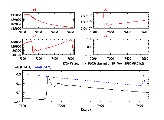
Figure 15.3 shows the online display of an EXAFS scan.
The upper half of the screen contains the counter readings, the lower half
shows the absorption of the sample which is compared with a reference
signal.
Figure 15.3:
The Online Display of EXAFS Scans
|
|